Frequency-dependent calibration

An example of how to use the frequency-dependent calibration functionality

• 
• 
• 

import scipy.signal as sig
import pathlib
import pyhydrophone as pyhy
import soundfile as sf
import numpy as np
import matplotlib.pyplot as plt

rtsys_name = 'RTSys'
rtsys_model = 'RESEA320'
rtsys_serial_number = 2003001
rtsys_sens = -180
rtsys_preamp = 0
rtsys_vpp = 5
mode = 'lowpower'
calibration_file = pathlib.Path("./../tests/test_data/rtsys/SN130.csv")
rtsys = pyhy.RTSys(name=rtsys_name, model=rtsys_model, serial_number=rtsys_serial_number, sensitivity=rtsys_sens,
                   preamp_gain=rtsys_preamp, Vpp=rtsys_vpp, mode=mode, calibration_file=calibration_file)

wav_path = './../tests/test_data/rtsys/channelA_2021-10-11_13-11-09.wav'
wav, fs = sf.read(wav_path)
frequencies, spectrum = sig.welch(wav, nfft=1024, scaling='density', fs=fs)
spectrum_db = 10 * np.log10(spectrum)
spectrum_db_upa = spectrum_db + rtsys.end_to_end_calibration()
frequency_increment = rtsys.freq_cal_inc(frequencies)
spectrum_db_upa_corrected = spectrum_db_upa + frequency_increment['inc_value']

plt.figure()
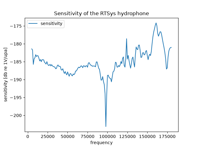
rtsys.freq_cal.plot('frequency', 'sensitivity')
plt.ylabel('sensitivity [db re 1V/upa]')
plt.title('Sensitivity of the RTSys hydrophone')
plt.show()

plt.figure()
plt.plot(frequencies, spectrum_db_upa, label='not corrected')
plt.plot(frequencies, spectrum_db_upa_corrected, label='corrected')
plt.legend()
plt.ylabel('Spectrum density [db re 1 upa**2/Hz]')
plt.xlabel('Frequency [Hz]')
plt.show()